In this post, I’ll demonstrate how to perform posterior inference for a basic
Gaussian Process (GP) regression model in various probabilistic programming
languages (PPLs). I will first start with a brief overview of GPs and their
utility in modeling functions. Check out the (free) GP for ML book by
Carl E. Rasmussen for more thorough explanations of GPs. Throughout the post, I
assume an understanding of basic supervised learning methods / techniques (like
linear regression and cross validation), and Bayesian methods.
Regression
In regression, one learns the relationship between a (possibly multivariate)
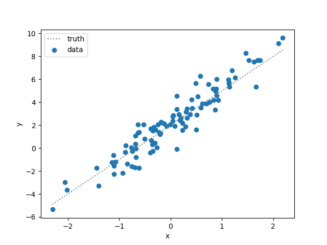
response $y_i$ and (one or more) predictors $X_i$. For example, the following
image shows the relationship between noisy univariate responses and predictors
(in dots); the dashed line shows that the true linear relationship response and
predictors.
A modeler interested in learning meaningful relationships between $y$ and
$X$ (possibly for a new, unobserved $X$) may choose to model this data with a
simple linear regression, in part due to its clear linear trend, as follows:
where $f(X_i) = \beta_0 + X_i \cdot \beta_1$ is a linear model, the model
parameters $\beta_0$ and $\beta_1$ are the intercept and slope, respectively;
and $\epsilon_i \sim \text{Normal}(0, \sigma^2)$, with another learnable model
parameter $\sigma^2$. One way to rewrite this model is
where $\boldsymbol{\beta} = (\beta_0, \beta_1)^T$, MvNormal denotes the
multivariate Normal distribution, and $\bm{I}$ is the identity matrix.
Because of the simplicity of this model and the data, learning the model
parameters is relatively easy.
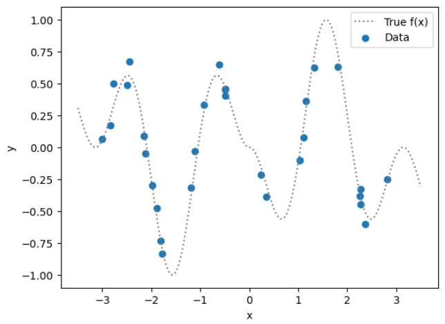
The following image shows data (dots) where the response $y$ and predictor $x$
have no clear relationship. The dashed line shows the true relationship between
$x$ and $y$, which can be viewed as a smooth (though non-trivial) function. A
linear regression will surely under fit in this scenario.
One of many ways to model this kind of data is via a Gaussian process (GP),
which directly models all the underlying function (in the function space).
A Gaussian process is a collection of random variables, any Gaussian process
finite number of which have a joint Gaussian distribution.
Note that the function $f(\bm{x})$ is distributed as a GP. For
simplicity (and for certain nice theoretical reasons), in many cases, constant
mean functions ($m(\bm{x})$ equals a constant) and covariance functions
that depend only on the distance $d$ between observations $\bm{x}$ and
$\bm{u}$ are used. When this is the case, another way to express a GP
model is
where $\bm{y}$ is a vector of length $N$ which contains the observed
responses; $\bm{X}$ is an $N\times P$ matrix of covariates; $m$ is a scalar
constant; $\bm{1}_N$ is a vector of ones of length $N$; and $K$ is an
$N\times N$ matrix such that $K_{i,j} = k(\bm{x}_i, \bm{x}_j)$. The
covariance function $k(\bm{x}, \bm{u})$ typically take on special
forms such that $K$ is a valid covariance matrix. Moreover, the covariance
function is often controlled by additional parameters which may control aspects
such as function smoothness and influence of data points on other data points.
For example, a common choice for the covariance function is the squared
exponential covariance function
which is parameterized by a covariance amplitude ($\alpha$) and range parameter
($\rho$). The range controls the correlation between two data points; larger
$\rho$, higher correlation for two data points for a fixed distance. Typically,
it is difficult to exactly specify these parameters, so they are estimated.
A natural way to do this is via a Bayesian framework, where prior information
about those parameters can be injected into the model.
A fully Bayesian model for the nonlinear data above can be specified as
follows:
Note that here, I’ve fixed the mean function to be 0, because the data is
somewhat centered there; but a constant mean function could be learned as well.
A Gaussian likelihood is used here, are observation-level noise is modeled
through $\sigma$. This enables one to marginalize over $\bm{f}$ analytically,
so that:
Note that for data with a different support, a different likelihood can be
used; however, the latent function $\bm{f}$ cannot in general be
analytically marginalized out.
The priors chosen need to be be somewhat
informative as there is not much information about the parameters from the data
alone. Here, the prior for $\alpha$ especially favors values near 1, which
means the GP variance will have an amplitude of around 1.
This model can be fit in the probabilistic programming languages (PPLs)
Turing, Stan, Pyro, Numpyro, and TFP via HMC, NUTS, and ADVI as follows:
# Import libraries.usingTuring,Turing:VariationalusingDistributionsusingAbstractGPs,KernelFunctionsimportRandomimportLinearAlgebra# NOTE: Import other libraries ...# NOTE: Read data ...# Define a kernel.sqexpkernel(alpha::Real,rho::Real)=alpha^2*transform(SqExponentialKernel(),1/(rho*sqrt(2)))# Define model.@modelGPRegression(y,X)=begin# Priors.alpha~LogNormal(0.0,0.1)rho~LogNormal(0.0,1.0)sigma~LogNormal(0.0,1.0)# Covariance function.kernel=sqexpkernel(alpha,rho)# GP (implicit zero-mean).gp=GP(kernel)# Sampling Distribution (MvNormal likelihood).y~gp(X,sigma^2+1e-6)# add 1e-6 for numerical stability.end;# Set random number generator seed.Random.seed!(0)# Model creation.m=GPRegression(y,X)# Fit via ADVI.q0=Variational.meanfield(m)# initialize variational distribution (optional)num_elbo_samples,max_iters=(1,2000)# Run optimizer.@timeq=vi(m,ADVI(num_elbo_samples,max_iters),q0,optimizer=Flux.ADAM(1e-1));# Fit via HMC.burn=1000nsamples=1000@timechain=sample(m,HMC(0.01,100),burn+nsamples)# start sampling.# Fit via NUTS.@timechain=beginnsamples=1000# number of MCMC samplesnadapt=1000# number of iterations to adapt tuning parameters in NUTSiterations=nsamples+nadapttarget_accept_ratio=0.8sample(m,NUTS(nadapt,target_accept_ratio,max_depth=10),iterations);end
# Import libraries ...
# Read data ...
# Define GP model.
gp_model_code="""
data {
int D; // number of features (dimensions of X)
int N; // number of observations
vector[N] y; // response
matrix[N, D] X; // predictors
// hyperparameters for GP covariance function range and scale.
real m_rho;
real<lower=0> s_rho;
real m_alpha;
real<lower=0> s_alpha;
real m_sigma;
real<lower=0> s_sigma;
}
transformed data {
// GP mean function.
vector[N] mu = rep_vector(0, N);
}
parameters {
real<lower=0> rho; // range parameter in GP covariance fn
real<lower=0> alpha; // covariance scale parameter in GP covariance fn
real<lower=0> sigma; // model sd
}
model {
matrix[N, N] K; // GP covariance matrix
matrix[N, N] LK; // cholesky of GP covariance matrix
rho ~ lognormal(m_rho, s_rho); // GP covariance function range parameter
alpha ~ lognormal(m_alpha, s_alpha); // GP covariance function scale parameter
sigma ~ lognormal(m_sigma, s_sigma); // model sd.
// Using exponential quadratic covariance function
// K(d) = alpha^2 * exp(-0.5 * (d/rho)^2)
K = cov_exp_quad(to_array_1d(X), alpha, rho);
// Add small values along diagonal elements for numerical stability.
for (n in 1:N) {
K[n, n] = K[n, n] + sigma^2;
}
// Cholesky of K (lower triangle).
LK = cholesky_decompose(K);
// GP likelihood.
y ~ multi_normal_cholesky(mu, LK);
}
"""# Compile model. This takes about a minute.
sm=pystan.StanModel(model_code=gp_model_code)# Data dictionary.
data=dict(y=y,X=X,N=y.shape[0],D=1,m_rho=0,s_rho=1.0,m_alpha=0,s_alpha=0.1,m_sigma=0,s_sigma=1)# Fit via ADVI.
vb_fit=sm.vb(data=data,iter=2000,seed=2,grad_samples=1,elbo_samples=1)vb_samples=pystan_vb_extract(vb_fit)# Fit via HMC
hmc_fit=sm.sampling(data=data,iter=2000,chains=1,warmup=1000,thin=1,seed=1,algorithm='HMC',control=dict(stepsize=0.01,int_time=1,adapt_engaged=False))# Fit via NUTS
nuts_fit=sm.sampling(data=data,iter=2000,chains=1,warmup=1000,thin=1,seed=1)
# NOTE: Import libraries...
# NOTE: Read data ...
# Default data type for tensorflow tensors.
dtype=np.float64# Set random seeds for reproducibility
np.random.seed(1)tf.random.set_seed(1)# Here we will use the squared exponential covariance function:
#
# $$
# \alpha^2 \cdot \exp\left\{-\frac{d^2}{2\rho^2}\right\}
# $$
#
# where $\alpha$ is the amplitude of the covariance, $\rho$ is the length scale
# which controls how slowly information decays with distance (larger $\rho$
# means information about a point can be used for data far away); and $d$ is
# the distance.
# Specify GP model
gp_model=tfd.JointDistributionNamed(dict(amplitude=tfd.LogNormal(dtype(0),dtype(0.1)),# amplitude
length_scale=tfd.LogNormal(dtype(0),dtype(1)),# length scale
v=tfd.LogNormal(dtype(0),dtype(1)),# model sd
obs=lambdalength_scale,amplitude,v:tfd.GaussianProcess(kernel=tfp.math.psd_kernels.ExponentiatedQuadratic(amplitude,length_scale),index_points=X[...,np.newaxis],observation_noise_variance=v)))# Run graph to make sure it works.
_=gp_model.sample()# Initial values.
initial_state=[1e-1*tf.ones([],dtype=np.float64,name='amplitude'),1e-1*tf.ones([],dtype=np.float64,name='length_scale'),1e-1*tf.ones([],dtype=np.float64,name='v')]# Bijectors (from unconstrained to constrained space)
bijectors=[tfp.bijectors.Softplus(),# amplitude
tfp.bijectors.Softplus(),# length_scale
tfp.bijectors.Softplus()# v
]# Unnormalized log posterior
defunnormalized_log_posterior(amplitude,length_scale,v):returngp_model.log_prob(amplitude=amplitude,length_scale=length_scale,v=v,obs=y)# Create a function to run HMC.
@tf.function(autograph=False)defrun_hmc(num_results,num_burnin_steps):returntfp.mcmc.sample_chain(num_results=num_results,num_burnin_steps=num_burnin_steps,current_state=initial_state,kernel=tfp.mcmc.SimpleStepSizeAdaptation(tfp.mcmc.TransformedTransitionKernel(inner_kernel=tfp.mcmc.HamiltonianMonteCarlo(target_log_prob_fn=unnormalized_log_posterior,step_size=0.01,num_leapfrog_steps=100),bijector=bijectors),num_adaptation_steps=num_burnin_steps),trace_fn=lambda_,pkr:pkr.inner_results.inner_results.is_accepted)# Run HMC.
[amplitudes,length_scales,v],is_accepted=run_hmc(1000,1000)# Create function to run NUTS.
@tf.function(autograph=False)defrun_nuts(num_results,num_burnin_steps):returntfp.mcmc.sample_chain(seed=1,num_results=num_results,num_burnin_steps=num_burnin_steps,current_state=initial_state,kernel=tfp.mcmc.SimpleStepSizeAdaptation(tfp.mcmc.TransformedTransitionKernel(inner_kernel=tfp.mcmc.NoUTurnSampler(target_log_prob_fn=unnormalized_log_posterior,max_tree_depth=10,step_size=0.1),bijector=bijectors),num_adaptation_steps=num_burnin_steps,target_accept_prob=0.8),trace_fn=lambda_,pkr:pkr.inner_results.inner_results.is_accepted)# Run NUTS.
[amplitudes,length_scales,v],is_accepted=run_nuts(1000,1000)### ADVI ###
# Create variational parameters.
qamp_loc=tf.Variable(tf.random.normal([],dtype=dtype)-1,name='qamp_loc')qamp_rho=tf.Variable(tf.random.normal([],dtype=dtype)-1,name='qamp_rho')qlength_loc=tf.Variable(tf.random.normal([],dtype=dtype),name='qlength_loc')qlength_rho=tf.Variable(tf.random.normal([],dtype=dtype),name='qlength_rho')qv_loc=tf.Variable(tf.random.normal([],dtype=dtype),name='qv_loc')qv_rho=tf.Variable(tf.random.normal([],dtype=dtype),name='qv_rho')# Create variational distribution.
surrogate_posterior=tfd.JointDistributionNamed(dict(amplitude=tfd.LogNormal(qamp_loc,tf.nn.softplus(qamp_rho)),length_scale=tfd.LogNormal(qlength_loc,tf.nn.softplus(qlength_rho))v=tfd.LogNormal(qv_loc,tf.nn.softplus(qv_rho))))# Function for running ADVI.
defrun_advi(sample_size,num_steps):returntfp.vi.fit_surrogate_posterior(target_log_prob_fn=unnormalized_log_posterior,surrogate_posterior=surrogate_posterior,optimizer=tf.optimizers.Adam(learning_rate=1e-2),seed=1,sample_size=sample_size,# ELBO samples.
num_steps=num_steps)# Number of iterations to run optimizer.
# Fit GP via ADVI.
losses=run_advi(sample_size=1,num_steps=2000)
# NOTE: Import library ...
# NOTE: Read Data ...
# Define GP Model
defmake_gp_model(X,y,length_prior=dist.LogNormal(0.0,1.0),variance_prior=dist.LogNormal(0.0,0.1),noise_prior=dist.LogNormal(0.0,1.0)):# Define squared exponential covariance function.
cov_fn=gp.kernels.RBF(input_dim=1)# Define GP regression model.
gpr=gp.models.GPRegression(X,y,cov_fn)# Place priors on GP covariance function parameters.
gpr.kernel.lengthscale=pyro.nn.PyroSample(length_prior)gpr.kernel.variance=pyro.nn.PyroSample(variance_prior)gpr.noise=pyro.nn.PyroSample(noise_prior)returngpr### HMC ###
pyro.clear_param_store()# Clear parameter cache.
pyro.set_rng_seed(1)# Set random seed for reproducibility.
hmc_gpr=make_gp_model(X,y)# Make GP model for HMC.
# Set up HMC sampler.
kernel=HMC(hmc_gpr.model,step_size=0.01,trajectory_length=1,target_accept_prob=0.8,adapt_step_size=False,adapt_mass_matrix=False)hmc=MCMC(kernel,num_samples=1000,warmup_steps=1000)hmc.run()# Run sampler.
hmc_posterior_samples=hmc.get_samples()# Get posterior samples
### NUTS ###
pyro.clear_param_store()pyro.set_rng_seed(1)nuts_gpr=make_gp_model(X,y)kernel=NUTS(nuts_gpr.model,target_accept_prob=0.8)nuts=MCMC(kernel,num_samples=1000,warmup_steps=1000)nuts.run()nuts_posterior_samples=nuts.get_samples()### ADVI ###
pyro.clear_param_store()# clear global parameter cache
pyro.set_rng_seed(1)# set random seed
# Automatically define variational distribution (a mean field guide).
guide=AutoDiagonalNormal(gp_model)# Create SVI object for optimization.
svi=SVI(gp_model,guide,Adam({'lr':1e-2}),JitTrace_ELBO())# Do 1000 gradient steps.
advi_loss=[]forstepintrange(1000):advi_loss.append(svi.step(X,y.double()))# Bijector for advi samples.
defbiject(samples):returndict(alpha=samples[:,0].exp().numpy(),rho=samples[:,1].exp().numpy(),sigma=samples[:,2].exp().numpy())# Get ADVI samples in constrained space.
advi_posterior_samples=biject(guide.get_posterior().sample((1000,)))
# NOTE: Import libraries ...
# One-dimensional squared exponential kernel with diagonal noise term.
defsquared_exp_cov_1D(X,variance,lengthscale):deltaXsq=np.power((X[:,None]-X)/lengthscale,2.0)K=variance*np.exp(-0.5*deltaXsq)returnK# GP model.
defGP(X,y):# Set informative log-normal priors on kernel hyperparameters.
variance=numpyro.sample("kernel_var",dist.LogNormal(0.0,0.1))lengthscale=numpyro.sample("kernel_length",dist.LogNormal(0.0,1.0))sigma=numpyro.sample("sigma",dist.LogNormal(0.0,1.0))# Compute kernel
K=squared_exp_cov_1D(X,variance,lengthscale)K+=np.eye(X.shape[0])*np.power(sigma,2)# Sample y according to the standard gaussian process formula
numpyro.sample("y",dist.MultivariateNormal(loc=np.zeros(X.shape[0]),covariance_matrix=K),obs=y)# Set random seed for reproducibility.
rng_key=random.PRNGKey(0)### Fit GP via HMC ###
# NOTE: num_leapfrog = trajectory_length / step_size
kernel=HMC(GP,step_size=.01,trajectory_length=1)hmc=MCMC(kernel,num_samples=1000,num_warmup=1000)hmc.run(rng_key,X,y)hmc_samples=hmc.get_samples()### Fit GP via NUTS ###
kernel=NUTS(GP,max_tree_depth=10,target_accept_prob=0.8nnuts=MCMC(kernel,num_samples=1000,num_warmup=1000)nuts.run(rng_key,X,y)nuts_samples=hmc.get_samples()## FIT GP via ADVI ###
# Setup
guide=AutoDiagonalNormal(GP)optimizer=numpyro.optim.Adam(step_size=0.01)svi=SVI(GP,guide,optimizer,loss=ELBO())init_state=svi.init(random.PRNGKey(1),X,y)# Run optimizer for 2000 iterations.
state,losses=lax.scan(lambdastate,i:svi.update(state,X,y),init_state,np.arange(2000))# Extract surrogate posterior.
params=svi.get_params(state)defsample_posterior(guide,params,nsamples,seed=1):samples=guide.get_posterior(params).sample(random.PRNGKey(seed),(nsamples,))# NOTE: Samples are arranged in alphabetical order.
# Not in the order in which they appear in the
# model. This is different from pyro.
returndict(rho=onp.exp(samples[:,0]),# kernel_length
alpha=onp.exp(samples[:,1]),# kernel_variance
sigma=onp.exp(samples[:,2]))# sigma
advi_samples=sample_posterior(guide,params,nsamples=1000,seed=1)
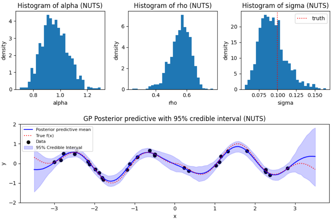
Posterior distributions
The parameters of interest here are the range, amplitude, and model standard
deviation parameters. The image below shows the posterior summaries of these
parameters obtained via NUTS in Turing. Posterior inference for the parameters
were similar across the different PPLs and inference algorithms. One is
typically interested in estimating the function $f$ over a (fine) grid of input
values, so included is the posterior distribution of $f$ (over a fine grid).
The shaded region is the 95% credible interval, the blue line is the posterior
mean function. The dashed line and dots are the posterior mean of the function
and data, respectively. Note how the credible interval for $f$ is narrower near
where data are observed, and wider when no data are nearby; that is,
uncertainty about the function is greater when you predict the output for
inputs about which you have less information.
Timings
The table below shows the compile and inference times (seconds) for each of the
PPLs and inference algorithms. (Smaller is better.) Note that the columns can
be sorted by clicking the column headers. The times shown here are the minimum
times from three runs for each algorithm and PPL.
PPL
ADVI (run)
HMC (run)
NUTS (run)
ADVI (compile)
HMC (compile)
NUTS (compile)
stan
0.187
10.9
0.683
54.7
54.7
54.7
turing
1.279
20.27
1.315
12.619
27.758
17.127
pyro
2.29
310.0
20.0
0.0
0.0
0.0
numpyro
1.57
18.0
7.0
0.235
2.9
1.11
tfp
2.76
81.0
14.4
0.0
2.44
4.1
Here are some details for the inference algorithm settings used:
ADVI
Number of ELBO samples was set to 1
Number of iterations was set to 2000
HMC
Step size = 0.01
Number of leapfrog steps = 100
Number of burn-in iterations = 1000
Number of subsequent samples collected = 1000
NUTS
Maximum tree depth = 10
Target acceptance rate = 80%
Adaptation / burn-in period = 1000 iterations
Number of sampler collected = 1000
The inference times for all algorithms are lowest in STAN. Pyro has the
largest inference times for HMC/NUTS (ADVI was not implemented). All
computations were done in a c5.xlarge AWS instance.