Gaussian Process Classification Model in various PPLs

This page was last updated on 29 Mar, 2021.


As a follow up to the previous post, this post demonstrates how Gaussian Process (GP) models for binary classification are specified in various probabilistic programming languages (PPLs), including Turing, STAN, tensorflow-probability, Pyro, Numpyro.

Data

We will use the following dataset for this tutorial.

data image

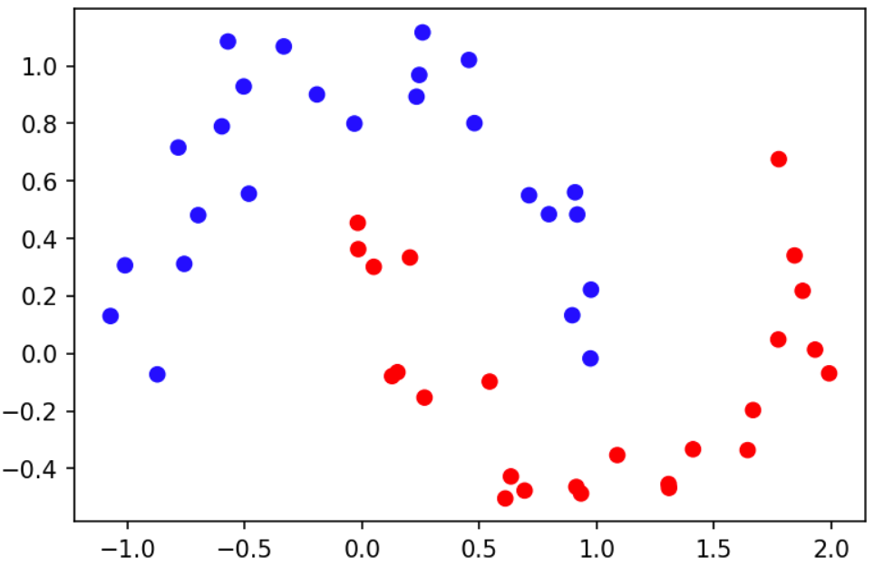
This dataset was generated using make_moons from the sklearn python library. The input ($X$) is a two-dimensional, and the response ($y$) is binary (blue=0, red=1). 25 responses are 0, and 25 response are 1. The goal, given this dataset, is to predict the response at new locations. We will use a GP binary classifier for this task.

Model

The model is specified as follows:

\[\begin{aligned} y_n \mid p_n &\sim \text{Bernoulli}(p_n), \text{ for } n=1,\dots, N &(1)\\ \text{logit}(\bm{p}) \mid \beta, \alpha, \rho &\sim \text{MvNormal}(\beta \cdot \bm{1}_N, \bm{K}_{\alpha, \rho}) &(2) \\ \beta &\sim \text{Normal(0, 1)} &(3) \\ \alpha &\sim \text{LogNormal}(0, 1) &(4)\\ \rho &\sim \text{LogNormal}(0, 1) &(5) \end{aligned}\]

We use a Bernoulli likelihood as the response is binary. We model the logit of the probabilities in the likelihood with a GP, with a $\beta$-mean mean function and squared-exponential covariance function, parameterized by amplitude $\alpha$ and range $\rho$, and with 2-dimensional predictors $x_i$. The finite-dimensional distribution can be expressed as in (2), where $K_{i,j}=\alpha^2 \cdot \exp\bc{-\norm{\bm{x}_i - \bm{x}_j}^2_2/2\rho^2}$. The model specification is completed by placing moderately informative priors on mean and covariance function parameters. For this (differentiable) model, full Bayesian inference can be done using generic inference algorithms (e.g.ADVI, HMC, and NUTS).

None of the PPLs explored currently support inference for full latent GPs with non-Gaussian likelihoods for ADVI/HMC/NUTS. (Though, some PPLs support variational inference via variational inference for sparse GPs, aka predictive processe GPs.) In addition, inference via ADVI/HMC/NUTS using the model specification as written above leads to slow mixing. Below is a reparameterized model which is (equivalent and) much easier to sample from using ADVI/HMC/NUTS. Note the introduction of auxiliary variables $\boldsymbol\eta$ to achieve this purpose.

\[\begin{aligned} y_n \mid p_n &\sim \text{Bernoulli}(p_n), \text{ for } n=1,\dots, N \\ \text{logit}(\bm{p}) &= \bm{L} \cdot \boldsymbol{\eta} + \beta\cdot\bm{1}_N, \text{ where } \bm{L} = \text{cholesky}(\bm{K}) \\ \eta_n &\sim \text{Normal(0, 1)}, \text{ for } n=1,\dots,N \\ \beta &\sim \text{Normal(0, 1)} \\ \alpha &\sim \text{LogNormal}(0, 1) \\ \rho &\sim \text{LogNormal}(0, 1) \end{aligned}\]

PPL Comparisons

Below are snippets of how this model is specified in Turing, STAN, TFP, Pyro, and Numpyro. Full examples are included in links above the snippets. The model was fit via ADVI, HMC, and NUTS for each PPL. The inferences were similar across each PPL via HMC and NUTS. The results were slightly different for $\alpha$ using ADVI, but were consistent across all PPLs. Below, we present posterior summaries for NUTS from Turing.

Full Turing Example (notebook)

1
2
3
4
5
6
7
8
9
10
11
12
13
14
15
16
17
18
19
20
21
22
23
24
25
26
27
28
29
30
31
32
33
34
35
36
37
38
39
40
41
42
43
44
45
46
47
48
49
50
51
52
53
54
55
56
57
58
59
60
61
62
63
64
65
66
67
68
69
70
71
72
73
74
75
76
77
78
79
80
81
82
83
84
85
86
87
88
89
90
91
92
93
94
95
96
97
# Import Libraries
using Turing
using Turing: Variational
using Distributions
using AbstractGPs, KernelFunctions
using PyPlot
using StatsFuns
using JSON3
using Flux
using ProgressBars
import Random
import LinearAlgebra

# Define a kernel.
sekernel(alpha, rho) = alpha^2 * transform(SEKernel(), invsqrt2/rho)

function compute_f(kernel, X, eta, beta=0, jitter=0)
  K = kernelmatrix(kernel, X, obsdim=1) + LinearAlgebra.I * jitter
  return LinearAlgebra.cholesky(K).L * eta .+ beta
end

@model function GPClassify(y, X, jitter=1e-6)
    # Priors.
    alpha ~ LogNormal(0, 1)
    rho ~ LogNormal(0, 1)
    beta ~ Normal(0, 1)  # intercept.
    eta ~ filldist(Normal(0, 1), length(y))

    # Latent GP
    kernel = sekernel(alpha, rho)
    f = compute_f(sekernel(alpha, rho), X, eta, beta, jitter)
    
    # Sampling Distribution.
    y ~ arraydist(Bernoulli.(logistic.(f)))
end;


# To extract parameters from trained variational distribution
# (surrogate posterior).
function make_surrogate_sampler(m, q; nsamples=300)
    qsamples = rand(q, nsamples)
    _, sym2range = Variational.bijector(m; sym_to_ranges=Val(true))
    return sym -> qsamples[collect(sym2range[sym][1]), :]
end;

### Read data ###
# See data in Notebook.
data_path = joinpath(@__DIR__, "../data/gp-classify-data-N50.json")

# Load data in JSON format.
data = let
    x = open(f -> read(f, String), data_path)
    JSON3.read(x)
end

### Name the data (X, y) ###
X = [data["x1"] data["x2"]]
y = Int64.(data["y"])

### Create model.###
m =  GPClassify(Float64.(y), X);
kernel_params = [:alpha, :rho, :beta];

### Fit via ADVI ###
Random.seed!(7)
@time q = vi(m, ADVI(1, 1000))  # num_elbo_samples, num_iterations.
 
# Get posterior samples
surrogate_sampler = make_surrogate_sampler(m, q, nsamples=500)
advi_samples = Dict{Symbol, Any}(sym => vec(surrogate_sampler(sym))
                                 for sym in kernel_params)
advi_samples[:eta] = extract_gp(:eta);

### Fit via HMC ###
Random.seed!(0)
burn = 500
nsamples = 500
@time hmc_chain = sample(m, HMC(0.05, 20), burn + nsamples);

# Get posterior samples
hmc_samples = Dict{Symbol, Any}([
    sym => vec(group(hmc_chain, sym).value.data)[end-nsamples+1:end]
for sym in kernel_params])
hmc_samples[:eta] = Matrix(group(hmc_chain, :eta).
                           value.data[end-nsamples+1:end, :, 1]')

### Fit via NUTS ###
Random.seed!(0)
burn = 500
nsamples = 500
@time nuts_chain = sample(m, NUTS(burn, 0.8, max_depth=10), burn + nsamples)

# Get posterior samples
nuts_samples = Dict{Symbol, Any}([
    sym => vec(group(nuts_chain, sym).value.data)
for sym in kernel_params])
nuts_samples[:eta] = Matrix(group(nuts_chain, :eta).value.data[:, :, 1]')

Full STAN Example (notebook)

1
2
3
4
5
6
7
8
9
10
11
12
13
14
15
16
17
18
19
20
21
22
23
24
25
26
27
28
29
30
31
32
33
34
35
36
37
38
39
40
41
42
43
44
45
46
47
48
49
50
51
52
53
54
55
56
57
58
59
60
61
62
63
64
65
66
67
68
69
70
71
72
73
74
75
76
77
78
79
80
81
82
83
84
85
86
87
88
89
90
91
92
93
94
95
96
97
98
99
100
101
102
103
104
105
106
107
108
109
110
# Load libraries.
import json
import numpy as np
import matplotlib.pyplot as plt
import pystan
from tqdm import trange
from scipy.spatial import distance_matrix
from scipy.stats import norm
from sklearn.datasets import make_moons
from sklearn.gaussian_process import GaussianProcessRegressor
from sklearn.gaussian_process.kernels import WhiteKernel, RBF


# Create data dictionary.
def create_stan_data(X, y, m_rho=0, s_rho=1, m_alpha=0, s_alpha=1, eps=1e-6):
    N, P = X.shape
    assert (N, ) == y.shape
    
    return dict(y=y, X=X, N=N, P=P,
                m_rho=m_rho, s_rho=s_rho,
                m_alpha=m_alpha, s_alpha=s_alpha, eps=eps)


# GP binary classification STAN model code.
model_code = """
data {
  int<lower=0> N;
  int<lower=0> P;
  int<lower=0, upper=1> y[N];
  matrix[N, P] X;
  real m_rho;
  real<lower=0> s_rho;
  real m_alpha;
  real<lower=0> s_alpha;
  real<lower=0> eps;
}

parameters {
  real<lower=0> rho;   // range parameter in GP covariance fn
  real<lower=0> alpha; // covariance scale parameter in GP covariance fn
  vector[N] eta;
  real beta;
}

transformed parameters {
  vector[N] f;
  {
    matrix[N, N] K;   // GP covariance matrix
    matrix[N, N] LK;  // cholesky of GP covariance matrix
    row_vector[N] row_x[N];
    
    // Using exponential quadratic covariance function
    for (n in 1:N) {
      row_x[n] = to_row_vector(X[n, :]);
    }
    K = cov_exp_quad(row_x, alpha, rho); 

    // Add small values along diagonal elements for numerical stability.
    for (n in 1:N) {
        K[n, n] = K[n, n] + eps;
    }

    // Cholesky of K (lower triangle).  
    LK = cholesky_decompose(K); 
  
    f = LK * eta;
  }
}

model {
  // Priors.
  alpha ~ lognormal(m_alpha, s_alpha);
  rho ~ lognormal(m_rho, s_rho);
  eta ~ std_normal();
  beta ~ std_normal();
 
  // Model.
  y ~ bernoulli_logit(beta + f);
}
"""


# Compile model. This takes about a minute.
sm = pystan.StanModel(model_code=model_code)


# Make data.
X, y = make_moons(n_samples=50, shuffle=True, noise=0.1, random_state=1)

# Generate stan data dictionary.
stan_data = create_stan_data(X, y)

# Fit via ADVI.
vb_fit = sm.vb(data=stan_data, iter=1000, seed=1,
               grad_samples=1, elbo_samples=1)

# Fit via HMC.
# - stepsize = 0.05
# - num leapfrog steps = 20
# - burn in: 500
# - samples: 500
hmc_fit = sm.sampling(
    data=stan_data, iter=1000, warmup=500, thin=1,
    seed=1, algorithm='HMC', chains=1,
    control=dict(stepsize=0.05, int_time=1, adapt_engaged=False))


# Fit via NUTS.
nuts_fit = sm.sampling(data=stan_data, iter=1000, warmup=500, thin=1,
                       seed=1, algorithm='NUTS', chains=1)

Full TFP Example (notebook)

1
2
3
4
5
6
7
8
9
10
11
12
13
14
15
16
17
18
19
20
21
22
23
24
25
26
27
28
29
30
31
32
33
34
35
36
37
38
39
40
41
42
43
44
45
46
47
48
49
50
51
52
53
54
55
56
57
58
59
60
61
62
63
64
65
66
67
68
69
70
71
72
73
74
75
76
77
78
79
80
81
82
83
84
85
86
87
88
89
90
91
92
93
94
95
96
97
98
99
100
101
102
103
104
105
106
107
108
109
110
111
112
113
114
115
116
117
118
119
120
121
122
123
124
125
126
127
128
129
130
131
132
133
134
135
136
137
138
139
140
141
142
143
144
145
146
147
148
149
150
151
152
153
154
155
156
157
158
159
160
161
162
163
164
165
166
167
168
169
170
171
172
173
174
175
176
177
178
179
180
181
182
183
184
185
186
187
188
189
190
191
# Import libraries.
import json
import numpy as np
import matplotlib.pyplot as plt
import tensorflow as tf
import tensorflow_probability as tfp
from tensorflow_probability import distributions as tfd
from tensorflow_probability import bijectors as tfb
from sklearn.datasets import make_moons
from tqdm import trange

sigmoid = lambda x: 1 / (1 + np.exp(-x))

# Alias.
SqExpKernel = tfp.math.psd_kernels.ExponentiatedQuadratic

# Default data type for tensorflow tensors.
dtype = np.float64

# Set random seeds for reproducibility
np.random.seed(1)
tf.random.set_seed(1)

# Read data
X, y = make_moons(n_samples=50, shuffle=True, noise=0.1, random_state=1)

# Store data.
X = np.stack([simdata['x1'], simdata['x2']], axis=-1).astype(dtype)
y = np.array(simdata['y'])


# Specify GP model.
def compute_LK(alpha, rho, X, jitter=1e-6):
    kernel = SqExpKernel(alpha, rho)
    K = kernel.matrix(X, X) + tf.eye(X.shape[0], dtype=dtype) * jitter
    return tf.linalg.cholesky(K)

def compute_f(alpha, rho, beta, eta):
    LK = compute_LK(alpha, rho, X)
    f = tf.linalg.matvec(LK, eta)  # LK * eta, (matrix * vector)
    return f + beta[..., tf.newaxis]

# GP Binary Classification Model.
gpc_model = tfd.JointDistributionNamed(dict(
    alpha=tfd.LogNormal(dtype(0), dtype(1)),
    rho=tfd.LogNormal(dtype(0), dtype(1)),
    beta=tfd.Normal(dtype(0), dtype(1)),
    eta=tfd.Sample(tfd.Normal(dtype(0), dtype(1)),
                   sample_shape=X.shape[0]),
    # NOTE: `Sample` and `Independent` resemble, respectively,
    # `filldist` and `arraydist` in Turing.
    obs=lambda alpha, rho, beta, eta: tfd.Independent(
        tfd.Bernoulli(logits=compute_f(alpha, rho, beta, eta)),
        reinterpreted_batch_ndims=1) 
))


### MODEL SET UP ###

# For some reason, this is needed for the compiler
# to know the correct model parameter dimensions.
_ = gpc_model.sample()


# Parameters as they appear in model definition.
# NOTE: Initial values should be defined in order appeared in model.
ordered_params = ['alpha', 'rho', 'beta', 'eta']

# Initial values.
tf.random.set_seed(1)
s = gpc_model.sample()
initial_state = [s[key] for key in ordered_params]

# Bijectors (from unconstrained to constrained space)
bijectors = [
    tfp.bijectors.Exp(),  # alpha
    tfp.bijectors.Exp(),  # rho
    tfp.bijectors.Identity(),  # beta
    tfp.bijectors.Identity(),  # eta
]

# Unnormalized log posterior
def unnormalized_log_posterior(alpha, rho, beta, eta):
    return gpc_model.log_prob(alpha=alpha, rho=rho,
                              beta=beta, eta=eta, obs=y)


### HMC ###
def hmc_trace_fn(state, pkr):
    """
    state: current state in MCMC
    pkr: previous kernel result
    """
    result = pkr.inner_results
    return dict(is_accepted=result.is_accepted,
                target_log_prob=result.accepted_results.target_log_prob)
    
@tfp.experimental.nn.util.tfcompile
def run_hmc(num_results, num_burnin_steps):
      return tfp.mcmc.sample_chain(
          num_results=num_results,
          num_burnin_steps=num_burnin_steps,
          current_state=initial_state,
          kernel=tfp.mcmc.TransformedTransitionKernel(
                     inner_kernel = tfp.mcmc.HamiltonianMonteCarlo(
                         target_log_prob_fn=unnormalized_log_posterior,
                         step_size=0.05,
                         num_leapfrog_steps=20),
                     bijector=bijectors),
          trace_fn=hmc_trace_fn)

# set random seed
tf.random.set_seed(2)
# Run HMC sampler
[alpha, rho, beta, eta], hmc_stats = run_hmc(500, 500)


### NUTS ###
def nuts_trace_fn(state, pkr):
    """
    state: current state in MCMC
    pkr: previous kernel result
    """
    result = pkr.inner_results.inner_results
    return dict(is_accepted=result.is_accepted,
                target_log_prob=result.target_log_prob)
  
@tfp.experimental.nn.util.tfcompile
def run_nuts(num_results, num_burnin_steps):
      return tfp.mcmc.sample_chain(
          num_results=num_results,
          num_burnin_steps=num_burnin_steps,
          current_state=initial_state,
          kernel=tfp.mcmc.SimpleStepSizeAdaptation(
              tfp.mcmc.TransformedTransitionKernel(
                  inner_kernel = tfp.mcmc.NoUTurnSampler(
                      target_log_prob_fn=unnormalized_log_posterior,
                      max_tree_depth=10, step_size=0.05),
                  bijector=bijectors),
          num_adaptation_steps=num_burnin_steps,
          target_accept_prob=0.8),
          trace_fn=nuts_trace_fn)

# set random seed
tf.random.set_seed(2)
# Run NUTS sampler
[alpha, rho, beta, eta], nuts_stats = run_nuts(500, 500)


### ADVI ###
tf.random.set_seed(3)

# Create variational parameters.
vp_dict = dict()
for key in ordered_params:
    param_shape = gpc_model.model[key].event_shape
    vp_dict[f'q{key}_loc'] = tf.Variable(
        tf.random.normal(param_shape, dtype=dtype), name=f'q{key}_loc')
    vp_dict[f'q{key}_rho'] = tf.Variable(
        tf.random.normal(param_shape, dtype=dtype), name=f'q{key}_rho')
    
# Create variational distribution.
surrogate_family = dict(alpha=tfd.LogNormal, rho=tfd.LogNormal,
                        beta=tfd.Normal, eta=tfd.Normal)
surrogate_posterior_dict = {
    key: surrogate_family[key](vp_dict[f'q{key}_loc'],
                               tf.nn.softplus(vp_dict[f'q{key}_rho']))
    for key in ordered_params
}
surrogate_posterior_dict['eta'] = tfd.Independent(
    surrogate_posterior_dict['eta'], reinterpreted_batch_ndims=1)
surrogate_posterior = tfd.JointDistributionNamed(
    surrogate_posterior_dict
)
    
# Function for running ADVI.
def run_advi(sample_size, num_steps):
    return tfp.vi.fit_surrogate_posterior(
        target_log_prob_fn=unnormalized_log_posterior,
        surrogate_posterior=surrogate_posterior,
        optimizer=tf.optimizers.Adam(learning_rate=1e-1),
        seed=1,
        sample_size=sample_size,  # ELBO samples.
        num_steps=num_steps)  # Number of iterations to run optimizer.

# Fit GP via ADVI.
losses = run_advi(sample_size=10, num_steps=1000)

# Extract posterior samples from variational distributions.
advi_samples = surrogate_posterior.sample(500)
advi_samples = {k: advi_samples[k].numpy() for k in advi_samples}

Full Pyro Example (notebook)

1
2
3
4
5
6
7
8
9
10
11
12
13
14
15
16
17
18
19
20
21
22
23
24
25
26
27
28
29
30
31
32
33
34
35
36
37
38
39
40
41
42
43
44
45
46
47
48
49
50
51
52
53
54
55
56
57
58
59
60
61
62
63
64
65
66
67
68
69
70
71
72
73
74
75
76
77
78
79
80
81
82
83
84
85
86
87
88
89
90
91
92
93
94
95
96
97
98
99
100
101
102
# Import libraries.
import os
import sys
import json
import matplotlib.pyplot as plt
import numpy as np
import pyro
import pyro.distributions as dist
from pyro.infer.mcmc.api import MCMC
from pyro.infer.mcmc import NUTS, HMC
import torch
import torch.distributions.constraints as constraints
from torch.nn.functional import pad
from tqdm import trange
from sklearn.datasets import make_moons

# For ADVI
from pyro.infer import SVI, Trace_ELBO, TraceEnum_ELBO
from pyro.contrib.autoguide import AutoDiagonalNormal
from pyro.optim import Adam

# For GP
import pyro.contrib.gp as gp

# Default to double precision for torch objects.
torch.set_default_dtype(torch.float64)


# Make data.
X, y = make_moons(n_samples=50, shuffle=True, noise=0.1, random_state=1)
X = torch.from_numpy(X)
y = torch.from_numpy(y)


# Model definition.
def sq_exp_kernel(d, alpha, rho):
    return alpha * alpha * torch.exp(-0.5 * torch.pow(d / rho, 2))

def compute_f(alpha, rho, beta, eta, X):
    N = X.shape[0]
    D = torch.cdist(X, X)
    K = sq_exp_kernel(D, alpha, rho) + torch.eye(N) * 1e-6
    L = K.cholesky()
    return L.matmul(eta) + beta

# GP Binary Classifier.
def gpc(X, y):
    N = y.shape[0]
    
    # Priors.
    alpha = pyro.sample('alpha', dist.LogNormal(0, 1))
    rho = pyro.sample('rho', dist.LogNormal(0, 1))
    beta = pyro.sample('beta', dist.Normal(0, 1))

    with pyro.plate('latent_response', N):
        eta = pyro.sample('eta', dist.Normal(0, 1))

    # Latent function.
    f = compute_f(alpha, rho, beta, eta, X)
   
    with pyro.plate('response', N):
        pyro.sample('obs', dist.Bernoulli(logits=f), obs=y)


# HMC
pyro.clear_param_store()  # clear global parameter cache.
pyro.set_rng_seed(2) # set random number generator seed.
hmc = MCMC(HMC(gpc, step_size=0.05, trajectory_length=1,
               adapt_step_size=False, adapt_mass_matrix=False,
               jit_compile=True),
           num_samples=500, warmup_steps=500)  # sampler setup.
hmc.run(X, y.double())  # run mcmc
hmc_posterior_samples = hmc.get_samples()  # get posterior samples.


# NUTS
pyro.clear_param_store() 
pyro.set_rng_seed(2)
nuts = MCMC(NUTS(gpc, target_accept_prob=0.8, max_tree_depth=10,
                 jit_compile=True),
            num_samples=500, warmup_steps=500)
nuts.run(X, y.double())
nuts_posterior_samples = nuts.get_samples()


# ADVI
pyro.clear_param_store()  # clear global parameter cache
pyro.set_rng_seed(1)  # set random seed

# Automatically define variational distribution (a mean field guide).
guide = AutoDiagonalNormal(gpc)

# Create SVI object for optimization.
svi = SVI(gpc, guide, Adam({'lr': 1e-2}), TraceEnum_ELBO())

# Do 1000 gradient steps.
advi_loss = []
for step in trange(1000):
    advi_loss.append(svi.step(X, y.double()))

# NOTE: See notebook to see full example.

Full Numpyro Example (notebook)

1
2
3
4
5
6
7
8
9
10
11
12
13
14
15
16
17
18
19
20
21
22
23
24
25
26
27
28
29
30
31
32
33
34
35
36
37
38
39
40
41
42
43
44
45
46
47
48
49
50
51
52
53
54
55
56
57
58
59
60
61
62
63
64
65
66
67
68
69
70
71
72
73
74
75
76
77
78
79
80
81
82
83
84
85
86
87
88
89
90
91
92
93
94
95
96
97
98
99
100
101
102
103
104
105
106
107
108
# Import libraries.
import json
import matplotlib.pyplot as plt
from jax import random, lax
import jax.numpy as np
import numpyro
import numpyro.distributions as dist
from numpyro.infer.autoguide import AutoDiagonalNormal
from numpyro.infer import SVI, ELBO
from numpyro.infer import MCMC, NUTS, HMC
import numpy as onp
from sklearn.datasets import make_moons
from tqdm import trange

from sklearn.gaussian_process import GaussianProcessRegressor
from sklearn.gaussian_process.kernels import WhiteKernel, RBF

# Default to double precision.
numpyro.enable_x64()


### Make data ###
X, y = make_moons(n_samples=50, shuffle=True, noise=0.1, random_state=1)


### Define Model ###
def sq_exp_cov(X, alpha, rho):
    D = np.linalg.norm(X[:, None] - X, ord=2, axis=-1)
    return alpha * alpha * np.exp(-0.5 * np.power(D / rho, 2))

def compute_f(alpha, rho, beta, eta, X, jitter=1e-6):
    N = X.shape[0]
    K = sq_exp_cov(X, alpha, rho) + np.eye(N) * jitter
    L = np.linalg.cholesky(K)
    return np.matmul(L, eta) + beta

# GP Binary Classifier.
def GPC(X, y):
    N = y.shape[0]
    
    # Priors.
    alpha = numpyro.sample('alpha', dist.LogNormal(0, 1))
    rho = numpyro.sample('rho', dist.LogNormal(0, 1))
    beta = numpyro.sample('beta', dist.Normal(0, 1))
    eta = numpyro.sample('eta', dist.Normal(np.zeros(N), 1))

    # Latent function.
    f = compute_f(alpha, rho, beta, eta, X, 1e-3)
   
    # Likelihood.
    numpyro.sample('obs', dist.Bernoulli(logits=f), obs=y)


### HMC ###
# Set random seed for reproducibility.
rng_key = random.PRNGKey(0)
# NOTE: num_leapfrog = trajectory_length / step_size
hmc = MCMC(HMC(GPC, step_size=.05, trajectory_length=1,
               adapt_step_size=False, adapt_mass_matrix=False),
           num_samples=500, num_warmup=500)
hmc.run(rng_key, X, y)  # Run sampler
hmc_samples = hmc.get_samples()  # Store samples.


### NUTS ###
# Set random seed for reproducibility.
rng_key = random.PRNGKey(0)
nuts = MCMC(NUTS(GPC, target_accept_prob=0.8, max_tree_depth=10),
            num_samples=500, num_warmup=500)
nuts.run(rng_key, X, y)  # run sampler.
nuts_samples = nuts.get_samples() ## collect samplers.


### ADVI ###
# Learn more about ADVI in Numpyro here: 
#   http://num.pyro.ai/en/stable/svi.html

# Compile
guide = AutoDiagonalNormal(GPC)
optimizer = numpyro.optim.Adam(step_size=0.01)
svi = SVI(GPC, guide, optimizer, loss=ELBO())
init_state = svi.init(random.PRNGKey(1), X, y)

# Run optimizer for 1000 iteratons.
state, losses = lax.scan(lambda state, i: 
                         svi.update(state, X, y),
                         init_state, np.arange(1000))

# Extract surrogate posterior.
params = svi.get_params(state)
plt.plot(losses);

def sample_posterior(guide, params, nsamples, seed=1):
    samples = guide.get_posterior(params).sample(
        random.PRNGKey(seed), (nsamples, ))
    # NOTE: Samples are arranged in alphabetical order.
    #       Not in the order in which they appear in the
    #       model. This is different from pyro.
    return dict(alpha=onp.exp(samples[:, 0]),
                beta=samples[:, 1],
                eta=samples[:, 2:52],
                rho=onp.exp(samples[:, -1]))

advi_samples = sample_posterior(guide, params,
                                nsamples=500, seed=1)


# NOTE: See notebook to see full example.

Here are some algorithm settings used for inference:

  • ADVI
    • Number of ELBO samples was set to 1
    • Number of iterations was set to 1000
    • Number of samples drawn from variational posterior distribution = 500
  • HMC
    • Step size = 0.05
    • Number of leapfrog steps = 20
    • Number of burn-in iterations = 500
    • Number of subsequent samples collected = 500
  • NUTS
    • Maximum tree depth = 10
    • Target acceptance rate = 80%
    • Adaptation / burn-in period = 500 iterations
    • Number of sampler collected = 500

Results

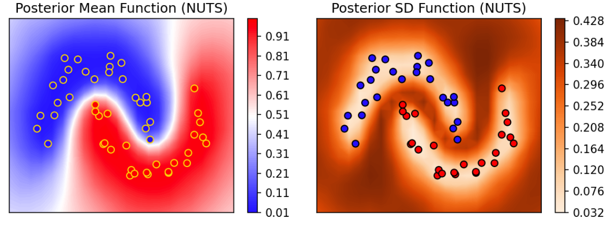
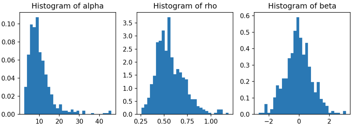
Below, the top left figure is the posterior predictive mean function $\bm{p}$ over a fine location grid. The data is included for reference. Note that where data-response is predominantly 0 (blue), the probability of predicting 0 is high (indicated by low probability of predicting 1 at those locations). Similarly, where data-response is predominantly 1 (red), the probability of predicting 1 is high. In the regions between, the probability of predicting 1 is near 0.5. The top right figure shows that where there is ample data, uncertainty (described via posterior predictive standard deviation) is low (whiter hue); and where data is lacking, uncertainty is high (darker hue). The bottom three panels show the posterior distribution of the GP parameters, $(\rho, \alpha, \beta)$.

UQ for GP classification

kerenl parameters posterior

Note that one shortcoming of Turing, TFP, Pyro, and Numpyro is that the latent function $f$ is not returned as posterior samples. Rather, due to the way the model is specified, only $\eta$ is returned. This means that $f$ needs to be recomputed. The re-computation of $f$ is not too onerous as the time spent doing posterior prediction is dominated by the required matrix inversions (or more efficient/stable variants using cholesky decompositions). Note that in STAN, posterior samples of $f$ can be obtained using the transformed parameters block.

Timings

Here we summarize timings for each aforementioned inference algorithm and PPL. Timings can be sorted by clicking the column-headers. The inference times for all algorithms are lowest in STAN. Turing has the highest inference times for all inference algorithms. All computations were done in a c5.xlarge AWS instance.

PPL ADVI (run) HMC (run) NUTS (run) ADVI (compile) HMC (compile) NUTS (compile)
stan 0.399 3.83 7.2 56.2 56.2 56.2
turing 13.176 64.383 102.772 15.272 20.159 11.685
pyro 5.0 31.0 73.0 0.0 0.0 0.0
numpyro 4.59 10.0 18.0 0.338 5.2 0.6
tfp 3.11 8.71 52.0 0.0 2.84 4.54