Dirichlet Process Gaussian mixture model via the stick-breaking construction in various PPLs
This page was last updated on 29 Mar, 2021.
In this post, I’ll explore implementing posterior inference for Dirichlet
process Gaussian mixture models (GMMs) via the stick-breaking construction in
various probabilistic programming languages. For an overview of the Dirichlet
process (DP) and Chinese restaurant process (CRP), visit this post on
Probabilistic Modeling using the Infinite Mixture Model by the Turing
team. Basic familiarity with Gaussian mixture models and Bayesian methods
are assumed in this post. This Coursera Course on Mixture Models offers a
great intro on the subject.
Note that this is a collapsed version of a DP (Gaussian) mixture model. Line 4
is the sampling distribution or model, where each of $N$ real univariate
observations ($y_i$) are assumed to be Normally distributed; line 3 are
independent priors for the mixture locations and scales. For example, the
distribution $G$ could be $\t{Normal}(\cdot \mid m, s) \times \t{Gamma}(\cdot
\mid a, b)$; i.e. a bivariate distribution with independent components – one
Normal and one Gamma. The CRP allows for the number of mixture components to be
unbounded (though it is practically bounded by $N$), hence $k=1,\dots,\infty$.
Line 2 is the prior for the cluster membership indicators. Through $z_i$, the
data can be partitioned (i.e. grouped) into clusters; Line 1 is an optional
prior for the concentration parameter $\alpha$ which influences the number of
clusters; larger $\alpha$, greater number of clusters. Note that the data
usually does not contain much information about $\alpha$, so priors for
$\alpha$ need to be at least moderately informative.
This model is difficult to implement generically in PPLs because it line 1
allows the number of mixture components (i.e. the dimensions of $\mu$ and
$\sigma$) to vary, and line 2 contains discrete parameters. It is true that for
a particular class of DP mixture models (for carefully chosen priors),
efficient posterior inference is just a matter of iterative and direct sampling
from full conditionals. But this convenience is not available in general, and
we still have the issue of varying number of mixture components. The PPL NIMBLE
(in R) addresses this issue by allowing the user to specify a maximum number of
components, it also cleverly exploits conjugate priors when possible. This
feature is not typically seen in PPLs, including Turing (at the moment). NIMBLE
also supports the sampling of discrete parameters, which is uncommon in PPLs
which usually implement generic and efficient sampling algorithms like HMC and
NUTS for continuous parameters. Turing supports the sampling of discrete
parameters via sequential Monte Carlo (SMC) and particle Gibbs (PG) /
conditional SMC.
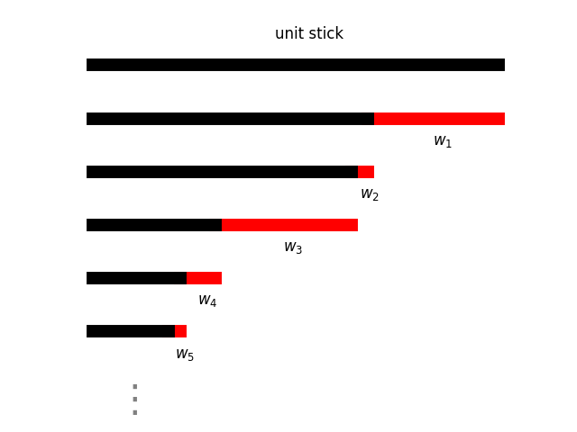
Having said that, the finite stick-breaking construction of the DP bypasses
the need for varying number of mixture components. In the context of mixture
models, the infinite stick-breaking construction of the DP constructs
mixture weights $(w_1, w_2, \dots)$ as follows:
This image shows a realization of $\bm{w}$ from the stick-breaking process
with $\alpha=3$.
Infinite probability vectors ($\bm{w}$) generated from this construction
are equivalent to the weights implied by the CRP (with parameter $\alpha$).
Hence, the probability vector $\bm{w}$ (aka simplex), where each element is
non-negative and the elements sum to 1, will be sparse. That is, most of the
weights will be extremely close to 0, and only a handful will be noticeably (to
substantially) greater than 0. The sparsity will be influenced by $\alpha$. In
practice, a truncated (or finite) version of the stick-breaking
construction is used. (An infinite array cannot be created on a computer…)
The finite stick-breaking model simply places an upper bound on the number of
mixture components, which, if chosen reasonably, allows us to reap the benefits
of the DP (a model which allows model complexity to grow with data size) at a
cheaper computational cost. The finite version is as follows:
Note that $w_K$ is defined such that $w_K = 1 - \sum_{k=1}^{K-1} w_k$. But
line 4 above is typically implemented in software for numerical stability.
Here on, for brevity, $\bm{w} = \t{stickbreak}(\bm{v})$ will denote the
transformation lines 2-4 above. Notice that the probability vector
$\bm{w}$ is $K$-dimensional, while $v$ is $(K-1)$-dimensional. (A simplex
$\bm{w}$ of length $K$ only requires $K-1$ elements to be specified. The
remaining element is constrained such that the probability vector sums to 1.)
A DP GMM under the stick-breaking construction can thus be specified as
follows:
where $G_\mu$ and $G_\sigma$ are appropriate priors for $\mu_k$ and $\sigma_k$,
respectively. Marginalizing over the (discrete) cluster membership indicators
$\bm{z}$ may be beneficial in practice if an efficient posterior inference
algorithm (e.g. ADVI, HMC, NUTS) exists for learning the joint
posterior of the remaining model parameters. If this is the case, one further
reduction can be made to yield:
The joint posterior of the parameters $\bm{\theta} = \p{\bm{\mu},
\bm{\sigma}, \bm{v}, \alpha}$ can be sampled from using NUTS or HMC, or
approximated via ADVI. This can be done in the various PPLs as follows. (Note that
these are excerpts from complete examples which are also linked.)
# NOTE: Import libraries here ...# DP GMM model under stick-breaking construction@modeldp_gmm_sb(y,K)=beginnobs=length(y)mu~filldist(Normal(0,3),K)sig~filldist(Gamma(1,1/10),K)# mean = 0.1alpha~Gamma(1,1/10)# mean = 0.1crm=DirichletProcess(alpha)v~filldist(StickBreakingProcess(crm),K-1)eta=stickbreak(v)y.~UnivariateGMM(mu,sig,Categorical(eta))end# NOTE: Read data y here ...# Here, y (a vector of length 500) is noisy univariate draws from a# mixture distribution with 4 components.# Fit DP-SB-GMM with ADVIadvi=ADVI(1,2000)# num_elbo_samples, max_itersq=vi(dp_gmm_sb(y,10),advi,optimizer=Flux.ADAM(1e-2));# Fit DP-SB-GMM with HMChmc_chain=sample(dp_gmm_sb(y,500),# data, number of mixture componentsHMC(0.01,100),# stepsize, number of leapfrog steps1000)# iterations# Fit DP-SB-GMM with NUTS@timenuts_chain=beginn_samples=500# number of MCMC samplesnadapt=500# number of iterations to adapt tuning parameters in NUTSiterations=n_samples+nadapttarget_accept_ratio=0.8sample(dp_gmm_sb(y,10),# data, number of mixture components.NUTS(nadapt,target_accept_ratio,max_depth=10),iterations);end
# import libraries here ...
model="""
data {
int<lower=0> K; // Number of cluster
int<lower=0> N; // Number of observations
real y[N]; // observations
real<lower=0> alpha_shape;
real<lower=0> alpha_rate;
real<lower=0> sigma_shape;
real<lower=0> sigma_rate;
}
parameters {
real mu[K]; // cluster means
// real <lower=0,upper=1> v[K - 1]; // stickbreak components
vector<lower=0,upper=1>[K - 1] v; // stickbreak components
real<lower=0> sigma[K]; // error scale
real<lower=0> alpha; // hyper prior DP(alpha, base)
}
transformed parameters {
simplex[K] eta;
vector<lower=0,upper=1>[K - 1] cumprod_one_minus_v;
cumprod_one_minus_v = exp(cumulative_sum(log1m(v)));
eta[1] = v[1];
eta[2:(K-1)] = v[2:(K-1)] .* cumprod_one_minus_v[1:(K-2)];
eta[K] = cumprod_one_minus_v[K - 1];
}
model {
real ps[K];
// real alpha = 1;
alpha ~ gamma(alpha_shape, alpha_rate); // mean = a/b = shape/rate
sigma ~ gamma(sigma_shape, sigma_rate);
mu ~ normal(0, 3);
v ~ beta(1, alpha);
for(i in 1:N){
for(k in 1:K){
ps[k] = log(eta[k]) + normal_lpdf(y[i] | mu[k], sigma[k]);
}
target += log_sum_exp(ps);
}
}
generated quantities {
real ll;
real ps_[K];
ll = 0;
for(i in 1:N){
for(k in 1:K){
ps_[k] = log(eta[k]) + normal_lpdf(y[i] | mu[k], sigma[k]);
}
ll += log_sum_exp(ps_);
}
}
"""# Compile the stan model.
sm=pystan.StanModel(model_code=model)# NOTE: Read data y here ...
# Here, y (a vector of length 500) is noisy univariate draws from a
# mixture distribution with 4 components.
# Construct data dictionary.
data=dict(y=simdata['y'],K=10,N=len(simdata['y']),alpha_shape=1,alpha_rate=10,sigma_shape=1,sigma_rate=10)# Approximate posterior via ADVI
# - ADVI is sensitive to starting values. Should run several times and pick run
# that has best fit (e.g. highest ELBO / logliklihood).
# - Variational inference works better with more data. Inference is less accurate
# with small datasets, due to the variational approximation.
fit=sm.vb(data=data,iter=1000,seed=1,algorithm='meanfield',adapt_iter=1000,verbose=False,grad_samples=1,elbo_samples=100,adapt_engaged=True,output_samples=1000)### Settings for MCMC ###
burn=500# Number of burn in iterations
nsamples=500# Number of sampels to keep
niters=burn+nsamples# Number of MCMC (HMC / NUTS) iterations in total
# Sample from posterior via HMC
# NOTE: num_leapfrog = int_time / stepsize.
hmc_fit=sm.sampling(data=data,iter=niters,chains=1,warmup=burn,thin=1,seed=1,algorithm='HMC',control=dict(stepsize=0.01,int_time=1,adapt_engaged=False))# Sample from posterior via NUTS
nuts_fit=sm.sampling(data=data,iter=niters,chains=1,warmup=burn,thin=1,seed=1)
# import libraries here ...
# Stickbreak function
defstickbreak(v):batch_ndims=len(v.shape)-1cumprod_one_minus_v=tf.math.cumprod(1-v,axis=-1)one_v=tf.pad(v,[[0,0]]*batch_ndims+[[0,1]],"CONSTANT",constant_values=1)c_one=tf.pad(cumprod_one_minus_v,[[0,0]]*batch_ndims+[[1,0]],"CONSTANT",constant_values=1)returnone_v*c_one# See: https://www.tensorflow.org/probability/api_docs/python/tfp/distributions/MixtureSameFamily
# See: https://www.tensorflow.org/probability/examples/Bayesian_Gaussian_Mixture_Model
# Define model builder.
defcreate_dp_sb_gmm(nobs,K,dtype=np.float64):returntfd.JointDistributionNamed(dict(# Mixture means
mu=tfd.Independent(tfd.Normal(np.zeros(K,dtype),3),reinterpreted_batch_ndims=1),# Mixture scales
sigma=tfd.Independent(tfd.LogNormal(loc=np.full(K,-2,dtype),scale=0.5),reinterpreted_batch_ndims=1),# Mixture weights (stick-breaking construction)
alpha=tfd.Gamma(concentration=np.float64(1.0),rate=10.0),v=lambdaalpha:tfd.Independent(# tfd.Beta(np.ones(K - 1, dtype), alpha),
# NOTE: Dave Moore suggests doing this instead, to ensure
# that a batch dimension in alpha doesn't conflict with
# the other parameters.
tfd.Beta(np.ones(K-1,dtype),alpha[...,tf.newaxis]),reinterpreted_batch_ndims=1),# Observations (likelihood)
obs=lambdamu,sigma,v:tfd.Sample(tfd.MixtureSameFamily(# This will be marginalized over.
mixture_distribution=tfd.Categorical(probs=stickbreak(v)),# mixture_distribution=tfd.Categorical(probs=v),
components_distribution=tfd.Normal(mu,sigma)),sample_shape=nobs)))# Number of mixture components.
ncomponents=10# Create model.
model=create_dp_sb_gmm(nobs=len(simdata['y']),K=ncomponents)# Define log unnormalized joint posterior density.
deftarget_log_prob_fn(mu,sigma,alpha,v):returnmodel.log_prob(obs=y,mu=mu,sigma=sigma,alpha=alpha,v=v)# NOTE: Read data y here ...
# Here, y (a vector of length 500) is noisy univariate draws from a
# mixture distribution with 4 components.
### ADVI ###
# Prep work for ADVI. Credit: Thanks to Dave Moore at BayesFlow for helping
# with the implementation!
# ADVI is quite sensitive to initial distritbution.
tf.random.set_seed(7)# 7
# Create variational parameters.
qmu_loc=tf.Variable(tf.random.normal([ncomponents],dtype=np.float64)*3,name='qmu_loc')qmu_rho=tf.Variable(tf.random.normal([ncomponents],dtype=np.float64)*2,name='qmu_rho')qsigma_loc=tf.Variable(tf.random.normal([ncomponents],dtype=np.float64)-2,name='qsigma_loc')qsigma_rho=tf.Variable(tf.random.normal([ncomponents],dtype=np.float64)-2,name='qsigma_rho')qv_loc=tf.Variable(tf.random.normal([ncomponents-1],dtype=np.float64)-2,name='qv_loc')qv_rho=tf.Variable(tf.random.normal([ncomponents-1],dtype=np.float64)-1,name='qv_rho')qalpha_loc=tf.Variable(tf.random.normal([],dtype=np.float64),name='qalpha_loc')qalpha_rho=tf.Variable(tf.random.normal([],dtype=np.float64),name='qalpha_rho')# Create variational distribution.
surrogate_posterior=tfd.JointDistributionNamed(dict(# qmu
mu=tfd.Independent(tfd.Normal(qmu_loc,tf.nn.softplus(qmu_rho)),reinterpreted_batch_ndims=1),# qsigma
sigma=tfd.Independent(tfd.LogNormal(qsigma_loc,tf.nn.softplus(qsigma_rho)),reinterpreted_batch_ndims=1),# qv
v=tfd.Independent(tfd.LogitNormal(qv_loc,tf.nn.softplus(qv_rho)),reinterpreted_batch_ndims=1),# qalpha
alpha=tfd.LogNormal(qalpha_loc,tf.nn.softplus(qalpha_rho))))# Run ADVI.
losses=tfp.vi.fit_surrogate_posterior(target_log_prob_fn=target_log_prob_fn,surrogate_posterior=surrogate_posterior,optimizer=tf.optimizers.Adam(learning_rate=1e-2),sample_size=100,seed=1,num_steps=2000)# 9 seconds
### MCMC (HMC/NUTS) ###
# Creates initial values for HMC, NUTS.
defgenerate_initial_state(seed=None):tf.random.set_seed(seed)return[tf.zeros(ncomponents,dtype,name='mu'),tf.ones(ncomponents,dtype,name='sigma')*0.1,tf.ones([],dtype,name='alpha')*0.5,tf.fill(ncomponents-1,value=np.float64(0.5),name='v')]# Create bijectors to transform unconstrained to and from constrained
# parameters-space. For example, if X ~ Exponential(theta), then X is
# constrained to be positive. A transformation that puts X onto an
# unconstrained # space is Y = log(X). In that case, the bijector used should
# be the **inverse-transform**, which is exp(.) (i.e. so that X = exp(Y)).
#
# NOTE: Define the inverse-transforms for each parameter in sequence.
bijectors=[tfb.Identity(),# mu
tfb.Exp(),# sigma
tfb.Exp(),# alpha
tfb.Sigmoid()# v
]# Define HMC sampler.
@tf.function(autograph=False,experimental_compile=True)defhmc_sample(num_results,num_burnin_steps,current_state,step_size=0.01,num_leapfrog_steps=100):returntfp.mcmc.sample_chain(num_results=num_results,num_burnin_steps=num_burnin_steps,current_state=current_state,kernel=tfp.mcmc.SimpleStepSizeAdaptation(tfp.mcmc.TransformedTransitionKernel(inner_kernel=tfp.mcmc.HamiltonianMonteCarlo(target_log_prob_fn=target_log_prob_fn,step_size=step_size,num_leapfrog_steps=num_leapfrog_steps,seed=1),bijector=bijectors),num_adaptation_steps=num_burnin_steps),trace_fn=lambda_,pkr:pkr.inner_results.inner_results.is_accepted)# Define NUTS sampler.
@tf.function(autograph=False,experimental_compile=True)defnuts_sample(num_results,num_burnin_steps,current_state,max_tree_depth=10):returntfp.mcmc.sample_chain(num_results=num_results,num_burnin_steps=num_burnin_steps,current_state=current_state,kernel=tfp.mcmc.SimpleStepSizeAdaptation(tfp.mcmc.TransformedTransitionKernel(inner_kernel=tfp.mcmc.NoUTurnSampler(target_log_prob_fn=target_log_prob_fn,max_tree_depth=max_tree_depth,step_size=0.01,seed=1),bijector=bijectors),num_adaptation_steps=num_burnin_steps,# should be smaller than burn-in.
target_accept_prob=0.8),trace_fn=lambda_,pkr:pkr.inner_results.inner_results.is_accepted)# Run HMC sampler.
current_state=generate_initial_state()[mu,sigma,alpha,v],is_accepted=hmc_sample(500,500,current_state)hmc_output=dict(mu=mu,sigma=sigma,alpha=alpha,v=v,acceptance_rate=is_accepted.numpy().mean())# Run NUTS sampler.
current_state=generate_initial_state()[mu,sigma,alpha,v],is_accepted=nuts_sample(500,500,current_state)nuts_output=dict(mu=mu,sigma=sigma,alpha=alpha,v=v,acceptance_rate=is_accepted.numpy().mean())
# import libraries here ...
# Stick break function
# See: https://pyro.ai/examples/dirichlet_process_mixture.html
defstickbreak(v):cumprod_one_minus_v=torch.cumprod(1-v,dim=-1)one_v=pad(v,(0,1),value=1)c_one=pad(cumprod_one_minus_v,(1,0),value=1)returnone_v*c_one# See: https://pyro.ai/examples/gmm.html#
# See: https://pyro.ai/examples/dirichlet_process_mixture.html
# See: https://forum.pyro.ai/t/fitting-models-with-nuts-is-slow/1900
# DP SB GMM model.
# NOTE: In pyro, priors are assigned to parameters in the following manner:
#
# random_variable = pyro.sample('name_of_random_variable', some_distribution)
#
# Note that random variables appear on the left hand side of the `pyro.sample` statement.
# Data will appear *inside* the `pyro.sample` statement, via the obs argument.
#
# In this example, labels are explicitly mentioned. But they are, in fact, marginalized
# out automatically by pyro. Hence, they do not appear in the posterior samples.
#
# Both marginalized and auxiliary variabled versions are equally slow.
defdp_sb_gmm(y,num_components):# Cosntants
N=y.shape[0]K=num_components# Priors
# NOTE: In pyro, the Gamma distribution is parameterized with shape and rate.
# Hence, Gamma(shape, rate) => mean = shape/rate
alpha=pyro.sample('alpha',dist.Gamma(1,10))withpyro.plate('mixture_weights',K-1):v=pyro.sample('v',dist.Beta(1,alpha,K-1))eta=stickbreak(v)withpyro.plate('components',K):mu=pyro.sample('mu',dist.Normal(0.,3.))sigma=pyro.sample('sigma',dist.Gamma(1,10))withpyro.plate('data',N):label=pyro.sample('label',dist.Categorical(eta),infer={"enumerate":"parallel"})pyro.sample('obs',dist.Normal(mu[label],sigma[label]),obs=y)# NOTE: Read data y here ...
# Here, y (a vector of length 500) is noisy univariate draws from a
# mixture distribution with 4 components.
# Fit DP SB GMM via ADVI
# See: https://pyro.ai/examples/dirichlet_process_mixture.html
# Automatically define variational distribution (a mean field guide).
pyro.clear_param_store()# clear global parameter cache
guide=AutoDiagonalNormal(pyro.poutine.block(dp_sb_gmm,expose=['alpha','v','mu','sigma']))svi=SVI(dp_sb_gmm,guide,Adam({'lr':1e-2}),TraceEnum_ELBO())pyro.set_rng_seed(7)# set random seed
# Do gradient steps.
forstepinrange(2000):svi.step(y,10)# Fit DP SB GMM via HMC
pyro.clear_param_store()pyro.set_rng_seed(1)kernel=HMC(dp_sb_gmm,step_size=0.01,trajectory_length=1,target_accept_prob=0.8,adapt_step_size=False,adapt_mass_matrix=False)hmc=MCMC(kernel,num_samples=500,warmup_steps=500)hmc.run(y,10)# Fit DP SB GMM via NUTS
pyro.clear_param_store()pyro.set_rng_seed(1)kernel=NUTS(dp_sb_gmm,target_accept_prob=0.8)nuts=MCMC(kernel,num_samples=500,warmup_steps=500)nuts.run(y,10)
# import some libraries here...
# Stick break function
defstickbreak(v):batch_ndims=len(v.shape)-1cumprod_one_minus_v=np.exp(np.log1p(-v).cumsum(-1))one_v=np.pad(v,[[0,0]]*batch_ndims+[[0,1]],constant_values=1)c_one=np.pad(cumprod_one_minus_v,[[0,0]]*batch_ndims+[[1,0]],constant_values=1)returnone_v*c_one# Custom distribution: Mixture of normals.
# This implements the abstract class `dist.Distribution`.
classNormalMixture(dist.Distribution):support=constraints.real_vectordef__init__(self,mu,sigma,w):super(NormalMixture,self).__init__(event_shape=(1,))self.mu=muself.sigma=sigmaself.w=wdefsample(self,key,sample_shape=()):# it is enough to return an arbitrary sample with correct shape
returnnp.zeros(sample_shape+self.event_shape)deflog_prob(self,y,axis=-1):lp=dist.Normal(self.mu,self.sigma).log_prob(y)+np.log(self.w)returnlogsumexp(lp,axis=axis)# DP SB GMM model.
# NOTE: In numpyro, priors are assigned to parameters in the following manner:
#
# random_variable = numpyro.sample('name_of_random_variable', some_distribution)
#
# Note that random variables appear on the left hand side of the
# `numpyro.sample` statement. Data will appear *inside* the `numpyro.sample`
# statement, via the obs argument.
#
# In this example, labels are explicitly mentioned. But they are, in fact,
# marginalized out automatically by numpyro. Hence, they do not appear in the
# posterior samples.
defdp_sb_gmm(y,num_components):# Cosntants
N=y.shape[0]K=num_components# Priors
# NOTE: In numpyro, the Gamma distribution is parameterized with shape and
# rate. Hence, Gamma(shape, rate) => mean = shape/rate
alpha=numpyro.sample('alpha',dist.Gamma(1,10))withnumpyro.plate('mixture_weights',K-1):v=numpyro.sample('v',dist.Beta(1,alpha,K-1))eta=stickbreak(v)withnumpyro.plate('components',K):mu=numpyro.sample('mu',dist.Normal(0.,3.))sigma=numpyro.sample('sigma',dist.Gamma(1,10))withnumpyro.plate('data',N):numpyro.sample('obs',NormalMixture(mu[None,:],sigma[None,:],eta[None,:]),obs=y[:,None])# NOTE: Read data y here ...
# Here, y (a vector of length 200) is noisy univariate draws from a
# mixture distribution with 4 components.
# Set random seed for reproducibility.
rng_key=random.PRNGKey(0)# FIT DP SB GMM via HMC
# NOTE: num_leapfrog = trajectory_length / step_size
kernel=HMC(dp_sb_gmm,step_size=.01,trajectory_length=1)hmc=MCMC(kernel,num_samples=500,num_warmup=500)hmc.run(rng_key,y,10)hmc_samples=get_posterior_samples(hmc)# FIT DP SB GMM via NUTS
kernel=NUTS(dp_sb_gmm,max_tree_depth=10,target_accept_prob=0.8)nuts=MCMC(kernel,num_samples=500,num_warmup=500)nuts.run(rng_key,y,10)nuts_samples=get_posterior_samples(nuts)# FIT DP SB GMM via ADVI
sigmoid=lambdax:1/(1+onp.exp(-x))# Setup ADVI.
guide=AutoDiagonalNormal(dp_sb_gmm)# surrogate posterior
optimizer=numpyro.optim.Adam(step_size=0.01)# adam optimizer
svi=SVI(guide.model,guide,optimizer,loss=ELBO())# ELBO loss
init_state=svi.init(random.PRNGKey(2),y,10)# initial state
# Run optimizer
state,losses=lax.scan(lambdastate,i:svi.update(state,y,10),init_state,np.arange(2000))# Extract surrogate posterior.
params=svi.get_params(state)defsample_advi_posterior(guide,params,nsamples,seed=1):samples=guide.get_posterior(params).sample(random.PRNGKey(seed),(nsamples,))# NOTE: Samples are arranged in alphabetical order.
# Not in the order in which they appear in the
# model. This is different from pyro.
returndict(alpha=onp.exp(samples[:,0]),mu=onp.array(samples[:,1:11]).T,sigma=onp.exp(samples[:,11:21]).T,eta=onp.array(stickbreak(sigmoid(samples[:,21:]))).T)# v
advi_samples=sample_advi_posterior(guide,params,nsamples=500,seed=1)
ADVI, HMC, and NUTS are not supported in NIMBLE at the moment. Though,
the model can be implemented and posterior inference can be made via
alternative inference algorithms. See:
this NIMBLE example.
The purpose of this post is to compare various PPLs for this particular model.
That includes things like timings, inference quality, and syntax sugar.
Comparing inferences is difficult without overwhelming the reader with many
figures. Suffice it to say that , where possible, HMC and NUTS performed
similarly across the various PPLs. And some discrepancies occurred for ADVI.
(Full notebooks with visuals are provided here.) Nevertheless, I have
included some information of the data used, and inferences from ADVI in Turing
here. (The inferences from HMC and NUTS were not vastly different.)
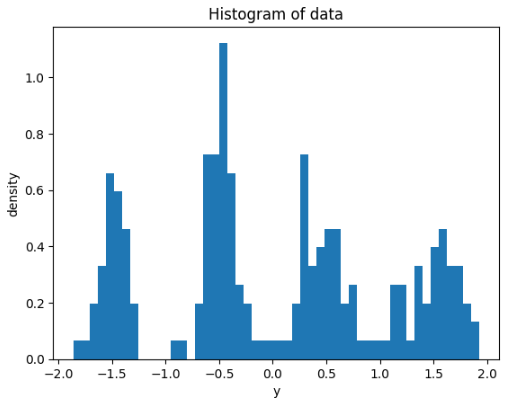
Here is a histogram of the data used. $y_i$ for $i=1,\dots,200$ is univariate
simulated from a mixture of four Normal distributions with varying locations
and scales. The specific dataset can be found here, and the scripts for
generating the data can be found here.
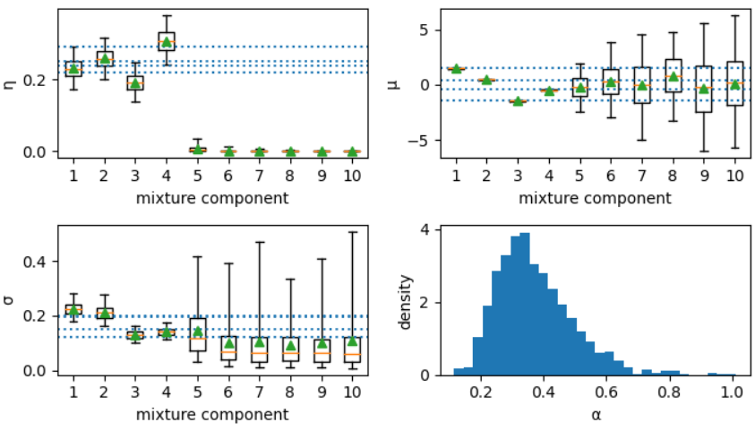
Here we have the posterior distributions of $\eta$ (the mixture weights, aka
$w$ above), $\mu$ (the mixture locations), $\sigma$ (the mixture scales),
and $\alpha$ the concentration parameter.
Note that the whiskers in the box plots are the ends of the 95% credible
intervals. The triangles and solid horizontal line in the boxplots are the
posterior means, and medians, respectively. The dashed lines are the simulation
truths, which match up closely to the posterior means, and fall within the 95%
credible intervals. Note for components 5-10, $\eta$ is near 0, due to the
sparse prior which is implied on it. In addition, $\mu$ and $\sigma$ for
components 5-10 are simply sampling from the prior, as no information is
available for those components (which are not used). The histogram for $\alpha$
is provided for reference. Since there is no simulation truth for $\alpha$, not
much more can be said about it. It is reasonable that it is in the range (0, 1)
due to the sparseness of the small number of mixture components and the prior
information. We can see that this model effectively learned there are only
4 clusters in this data.
Comparing the PPLs
First off, these are the settings used for HMC, and NUTS:
ADVI:
The optimizers for ADVI were run for 2000 iterations.
Full ADVI was done (i.e. no sub-sampling of the data as in stochastic
ADVI)
STAN defaults to using 100 samples for ELBO approximation
and 10 samples for ELBO gradient approximation. When I set these to 1,
like in Turing (and also recommended in the ADVI paper), the inferences
were quite bad, so I left them at the default. Nevertheless, STAN still
ran the fastest.
NOTE: ADVI is extremely sensitive to initial values. The best run from
multiple runs with varying initial values was used.
NOTE: There are discrepancies in the optimizers used in each PPL.
In Pyro and Turing, the Adam optimizer was used; in STAN, RmsProp was
used.
HMC
Step-size: 0.01
Number of leapfrog steps: 100
Number of burn-in iterations: 500
Number of subsequent HMC iterations: 500
This is also the number of posterior samples
NOTE: Relatively robust to initial values.
NUTS
Target acceptance rate: 80%
Number of iterations for burn-in: 500
NOTE: In TFP, the number of iterations for adapting NUTS
hyper-parameters was set to 400 (this needs to be less than the
burn-in, as it is part of the burn-in period).
Maximum tree-depth: 10
Number of subsequent NUTS iterations: 500
This is also the number of posterior samples
NOTE: Relatively robust to initial values.
Note: Automatic differentiation (AD) libraries used vary between the
PPLs. The default AD libraries in each PPL were used. This may have a
small effect on the timings.
Specifying the DP GMM via stick-breaking is quite simple in each of the PPLs.
Each PPL has also strengths and weaknesses for this particular model.
Particularly, some PPLs had shorter compile times; others had short
inference-times. It appears that the inferences from HMC and NUTS are similar
across the PPLs. Pyro implements ADVI, but the inferences were quite poor
compared to STAN, Turing, and TFP (several random initial values were used).
Numpyro was fastest at HMC and NUTS. STAN was fastest at ADVI, though it had
the longest compile time. (Note that the compile time for STAN models can be
one-time, as you can cache the compiled model.)
STAN, being the oldest of the PPLs, has the most comprehensive documentation.
So, implementing this particular model was quite easy.
TFP is quite verbose, but offers a lot of control for the user. I had some
difficulty getting the dimensions (batch_dim, event_shape) correct
initially. Dave Moore, who works at Google’s BayesFlow team, gracefully
looked at my code and offered fixes!
I would like to point out (while acknowledging my current affiliation with the
Turing team) the elegance of the syntax of Turing’s model specification. It is
close to how one would naturally write down the model, and it is also the
shortest. For those that are already familiar with Julia, custom functions
(such as the stickbreak function used) can be implemented by the user
and used in the model specification. Note that functions from other libraries
can be used quite effortlessly. For example, in Turing, the logsumexp and
normlogpdf methods are from the StatsFuns.jl library. They worked without
any tweaking in Turing. Another strength of Turing sampling from the full
conditionals of individual (or a group of) parameters using different inference
algorithms is possible. For example,
hmc_chain=sample(dp_gmm_sb(y,500),# data, number of mixture componentsGibbs(HMC(0.01,100,:mu,:sig,:v),MH(:alpha)),1000)# iterations
enables the sampling of $(\mu, \sigma, v)$ jointly conditioned on the current
$\alpha$, using HMC; and sampling $\alpha \mid
\bm{\mu},\bm{\sigma},\bm{v}$ via a vanilla Metropolis-Hastings
step. This is not possible in STAN, Pyro, Numpyro, and TFP. (This is also
possible in NIMBLE; however, NIMBLE currently does not support inference
algorithms based on AD.) Another possibility in Turing is:
hmc_chain=sample(dp_gmm_sb(y,500),# data, number of mixture componentsGibbs(HMC(0.01,100,:mu,:sig),HMC(0.01,100,:v),MH(:alpha)),1000)# iterations
where separate HMC samplers are used for $(\mu, \sigma)$ and $\bm{v}$.
For HMC, the inference timings of Turing are within an order of magnitude from
the fastest PPL (Numpyro). I think time and inference comparisons via HMC may
be fairer than the NUTS and ADVI comparisons as the implementations of HMC is
comparatively more well-defined (standardized) and relatively simple; whereas
the implementations of ADVI and NUTS are nuanced, and for NUTS quite complex.
As already stated, the quality of AD libraries will affect timings, and
possibly the quality of the inferences. Though the AD libraries used (Flux,
autodiff, torch, tensorflow, JAX) all seem rather robust.
Timings
Here are the compile and inference times (in seconds) for each PPL for this
model. Smaller is better. (By clicking the column headers, you can sort the
rows by inference times.)
PPL
ADVI (run)
HMC (run)
NUTS (run)
ADVI (compile)
HMC (compile)
NUTS (compile)
stan
2.3
23.3
99.0
52.3
52.3
52.3
turing
7.0
116.0
676.0
7.9
18.5
10.3
tfp
3.0
14.4
51.4
0.0
8.8
16.3
pyro
8.0
178.0
1106.0
0.0
0.0
0.0
numpyro
3.4
9.0
30.0
6.6
7.2
2.6
For STAN, the compile times listed is the time required to compile the model;
i.e. the time required to run this command:
sm=pystan.StanModel(model_code=model)
The model is compiled only once (and not three times), then the user is free to
select the inference algorithm.
The timings provided are one-off, but they don’t vary much from run-to-run, and
don’t affect the rankings of the PPLs in terms of speed for each inference
algorithm.
Note that for the Turing model, noticeable (40-60%) speedups can be realized by
replacing the UnivariateGMM model by a direct increment of the log
unnormalized joint posterior pdf. See this implementation and the results
timings.
The Manifest.toml and requirements.txt files, respectively, in the GitHub
project page list the specific Julia and Python libraries used for these
runs. All experiments for this project were done in an c5.xlarge AWS Spot
Instance. As of this writing, here are the specs for this instance:
vCPU: 4 Intel(R) Xeon(R) Platinum 8124M CPU @ 3.00GHz
RAM: 8 GB
Storage: EBS only (32 GB)
Network Bandwidth: Up to 10 Gbps
EBS Bandwidth: Up to 4750 Mbps
Next
In my next post, I will do a similar comparison of the PPLs and inference
algorithms mentioned here for a basic Gaussian process model.